Logion - A Robot Which Collects Rocks
mart@ksi.mff.cuni.cz,
david.obdrzalek@mff.cuni.cz
Abstract. In this paper[1] we present a design of autonomous robot built
for Eurobot 2008 contest by the MART team. We describe chosen strategy and the
way of its implementation, localization on the playing field using Monte Carlo
Localization and methods we use for moving the robot such as trajectory generation
mechanism and PID regulation.
Keywords: autonomous robot design,
MCL localization, PID regulation, robot navigation
1 Introduction
This paper
presents Logion – a robot build for Eurobot autonomous robot contest, namely
its 2008 edition with theme “
The robot (see
Fig. 1) has been designed and built by a student group at
Faculty of Mathematics and Physics,
The Eurobot
contest rules are different every year. However, basic attributes remain the
same over years: during a 90 sec match, two autonomous robots perform certain
tasks on a playing field in a friendly spirit. Specific topic is renewed every
year and requires general rework if a team wants to reuse its robot from
previous year. Therefore we decided to design the robot so that as many as
possible of its modules could be reused without dropping everything and
starting from scratch again.
For the
2008 edition, the theme is called “Mission to Mars”. The robots have to find
and collect “rock samples” (represented by coloured floorballs) and store them
in “containers for sample transfer back to the Earth” (represented by three
containers mounted on the outside border of the playing field). The samples may
be found laying on the “Mars surface” (the playing field floor) or in special
dispensers mounted on the playing field border.
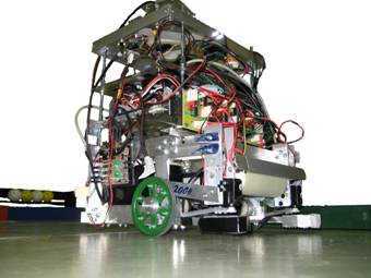
Fig. 1. Logion robot with its covers
removed
The rules
require the diameter to be at most 120 cm at start time and 140 cm at
any time during the match if the robot uses deployable mechanisms. The Logion
robot diameter stays nearly the same during the match with the only slight
exception concerning the ball extraction mechanism. This device is formed by
two “fingers” which rotate and pick balls from the vertical dispensers.
The robot
uses differential steering by two powered wheels with attached encoders
providing odometry information. The body is supported by one unpowered and uncontrolled
caster. Its mechanical construction consists of individual modules mounted
together in layers so that it can be dismounted and the modules reused for
further projects.
As we wanted to
use a lot of computing power (picture analysis, smart algorithms etc.) we
decided to use standard PC platform as the main computing unit. To use as much
computing power as the processor can offer, we powered the PC with Gentoo
Linux. Other advantage of using Linux is the ease of using the connected
hardware via nice and clear abstraction.
The top-level controlling software is
written in C++ with the use of object oriented programming. Kernel modules and
MCU firmware was written in C. Minor part of the project like monitoring over
the network was written in C#.
As the main features of the robot
controlling software we can talk about robot moving which use autopilot to
drive to absolute position, curves to plan routes trough the balls and avoid
opponent,
For more
technical reference, see Chapter 9 or MART team web pages [2].
In this section
we describe the main control part, which is responsible for the overall strategy
and its implementation. Therefore we call it the Brain.
The Brain
is driven by quite standard state machine (see Fig. 2). The states represent individual parts of the
robot’s mission. For example, the state “Extract samples” consists of a
sequence of actions which picks the ball from a vertical dispenser. This state
requires the robot to be well positioned in front of the dispenser, which is performed
by the state called “Go to dispenser” which selects the dispenser to go to and
makes the movement and positioning of the robot. When the robot collects five
balls (the limit set by the rules), the control is passed to the state “Go to
container”.
We wanted
to design the robot control to be robust. It was obvious the robot has to react
to situations which can appear without any dependence on the state. Therefore,
in addition to the state machine, we have created several triggers which are
repeatedly checked by the Brain. Such problematic situations include for example
the possible collision with the opponent’s robot or when the robot stucks after
unexpected bump to the border.
In case
such asynchronous situation occurs, the Brain switches from the actual state to
the specific situation handler. Based on the situation character and its
handler implementation, upon the handler completion the previously executed state
is restarted or the state machine is set to a state specified by the handler. To
implement this mechanism, a simple threading was used. The main Brain thread
controls the state switching and the special event checks. It performs only
non-blocking and fast operations. Individual operating state actions are called
in the BrainSlave thread. The main Brain thread may stop this slave at any time
and if it is needed, it may replace it by a thread performing action of a
different state. Fig. 2 shows the state machine without the asynchronous
event checks.
Fig. 2. The main state machine
To perform its tasks, the robot must be able to localize itself on the playing field. In the following paragraphs we present our approach.
We decided to use the already well
established
For reliable localization, we needed absolute information. For this purpose we tried to use an electronic compass CMPS03 [6]. But as we find later, such compass installed on a metal robot with electric motors is really faithless sensor. Motor activation changes the compass information for about 20 to 50 degrees away. Despite of this, the information still could be used, just very carefully. In MCL, we penalize only samples whose direction differs more than 90 degrees from the measurement.
As an
additional source for absolute positioning we have developed beacons. In
Eurobot 2008 edition, it was possible to use 4 beacons placed around the
playing field, at the opponent’s robot and on our robot. We have used three
active (transmitting) beacons around the playing field and one passive
(receiving) beacon on our robot (see their schematized positions on Fig. 3). Every active beacon transmits an infrared and an
ultrasonic signal at the same time. The passive beacon receives both signals
and based on the delay between them we can very precisely determine the distance
between the active and the passive beacons. To avoid false detection (e.g. from
opponent systems or from other surrounding noise), we use coded signal
(pulse-position modulation). We can determine if it is a signal transmitted
form our beacon and we can also identify which of our beacons is the transmitter.
Because of
the nature of ultrasonic signal, we cannot avoid false detection caused by the
signal rebounds. In fact, there were a lot of such rebounds in our lab. We had
therefore a good motivation to build a robust system for using information from
beacons. In one hand we have very good and precise information about distance
from a beacon (in real max ± 5 cm) while in the other hand we get false information sometimes.
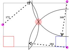
Fig. 3. Beacons
distance information (screenshot)
In our
first attempt we used this information in MCL in the simplest way. The beacon
signals were handled independently and we penalized the samples linearly according
to distance from a beacon every time we received the signal. This method has significant
disadvantage in case we are on a location where we receive a lot of rebounded
signals. In such situation all MCL samples move to that false radius.
As an
improvement, we combine the three beacon signals before the samples weights are
updated. In case we have received distance information from all three beacons during
short time and all three radiuses had one common intersection, we increased the
weight of MCL samples in close surrounding of the intersection and decreased
samples weight which were not close enough. If only two beacon signals arrive,
we use the two intersections of the two radiuses but in this case we updated
samples weight more carefully. And if we got only one radius we updated the
weights even more carefully. We decided not to use linear dependence anymore. If
the samples are not near the measured position, their weights are decreased by
constant and therefore samples are not affected by false information.
5 Moving
The Brain
manoeuvring mechanism (the Autopilot) uses a module called Driver which
provides complex API for controlling the robot move. For the Driver, we have
decided to create two driving methods which use absolute and relative movement,
respectively.
The first
method drives the robot to a certain place on the playing field when this place
is entered using absolute coordinates. For successful navigation with this moving
type, at least estimative position knowledge is needed. Two typical commands
for this method are “Go to position” and “Rotate to”.
The actual
movement was in this mode controlled by the Autopilot with the help of two
curves (see Fig. 4). One curve shows dependency between the speed and
the distance to the goal, the second curve shows dependency between the
difference of motors speeds and angular deviation of actual robot heading to
the desired heading.
Fig. 4. Autopilot control curves for
different robot weights: Speed to Distance (left),
Motors speed difference to Angular deviation (right)
The Autopilot
control functions are designed so that the robot slows down when approaching
the goal position and so can arrive to the required position more precisely
(this applies to both the x-y placement as well as the angular rotation of the
robot). Before the movement was implemented this way, the robot could exhibit
oscillation around the desired position because of its mass and the traction
characteristics.
Both curves
are defined by two parameters which should be set accordingly to the robot body
construction and should be recalibrated when the wheelframe is modified or when
the robot weight considerably changes.
The second
driving method is a relative movement. It is used for precise positioning of
the robot. We use this method for example to precisely adjust the robot in
front of the vertical dispenser before the robot tried to extract balls from
it. Another use for this method was to recover from robot blockage at the
border. In such a case, it is quite likely that we do not know the exact
position of the robot, otherwise we would not drive the robot so that it
collides with the border. Therefore the relative movement is the only right
style. Two typical command for this driving method are “Forward with speed“ and
“Rotate by“.
For speed
regulation we use standard proportional–integral–derivative (PID) controller. This controller
was implemented as one of the Driver functions. This decision allowed us to
generate very detailed outputs which were especially useful during the
fine-tuning of robot control parameters and for explaining its occasional
strange behaviour. We also considered the PID implementation to be set in the
lowest layer (in the HBmotor board MCU, which controlled directly the motor
rotation via regular H-bridge circuit; for details, see [2]), which could speed it significantly. However, looking
back, we think we made good decision. During the implementation process, we
have met with many different problems we were not aware of from the theory. For
example, we had to limit the derivative component as it could raise above all
reasonable values when the robot got stuck somewhere and after resolving of
that problem it took a very long time to decrease to normal values (which in
fact disallowed correct robot driving).
Basic PID
parameter setting was done based on Ziegler–Nichols method [7]. During the last phases of robot building, its
weight changed in the range of ± 8% which negatively affected the robot’s
smooth motion. Therefore the PID parameters had to be tuned to suit the new
situation. We did this tuning manually and thanks to the PID implementation in
the HW abstraction layer, it was possible to do it on the fly when the robot
was running on the playing field in square trajectory. At the same time, we
were able to see the direct impact of the change on the motion smoothness as
well as get the PID regulator graphs what would be hardly possible with the PID
regulation implemented in the lowest layer.
The
combination of Autopilot functions allows driving in non-trivial curves. Using
purely those functions, the motion would be limited to a simple point-to-point
navigation. However, as a result of the action planning, we are able to create
a list of successive sub-goals. It would be nice to be able to create a curve
that represents the optimal path trough all the sub-goals to the final
position. In case of Eurobot 2008 contest, that could be used for collecting
more balls on the table during one continuous motion and bringing them to the
destination container. As we will show in Chapter 7, it can be also used for collision avoidance by
simply inserting a new sub-goal into the goal list.
Simple
planning of the motion from one point to the next one is not feasible as it
does not guarantee smooth joints and the robot physically cannot make instant movement
changes. Therefore we had to seek more advanced algorithms than simple joining
of the curves and create one segmented curve with “nice behaviour”, at least to
provide continuous and smooth joins. We decided to use Hermite curves, because
these curves meet the expectations, are easily calculable and on the top of it,
they pass through their control points (see Fig. 5). To calculate one curve segment we need only to know
the positions and the tangents of its two endpoints. If more segments are
combined to create a joint curve and the tangents for the join points (the
“checkpoints”) are the same, the resulting curve meets our expectations. For
our purposes, it was even possible to make the tangents optional, which lets the
input to be really minimal.
Fig. 5. Examples of Hermite curves (P0, P1: control points, T0, T1: tangents)
The tangent
vectors can be sensed as analogous to the direction and speed of the curve at
that point. We have found that if we make the tangents always point to the next
checkpoint, we acquire reasonably good compound curve while minimizing inputs
for the calculations done by the Manoeuvre class. Its interface allows adding,
removing and changing of the curve checkpoints to form a queue. After we reach
the next checkpoint in the queue, it becomes the starting point. Fig. 6 shows an example of planned trajectory to collect all
balls detected on the playing field surface during the so-called “harvest” phase.
The ball positions are used as checkpoint and as such they define the curve
segments. If a new target is detected along the robot journey, it can be easily
added to the already existing list as a new checkpoint.
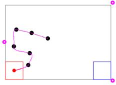
Fig. 6. Hermite curves used for balls harvest (screenshot)
The Mars rock samples are in the Eurobot contest located in three
principally different prospecting zones: on the surface, in one of the four vertical
dispensers (5 rock samples in each) and in one horizontal dispenser (12
samples). In this section we focus on the dispenser detection and exploitation.
The current
implementation of Logion robot does not use the horizontal dispenser. To pick
samples from the vertical dispensers, our robot has to be well-positioned in
front of it. We can acquire a good localization from our beacons data, but they
cannot tell us the robot heading. Information about the angle is corrected by
In the
game, the dispensers are made using transparent plastic sheet and the balls in a
dispenser can be easily seen through it. Therefore we decided to use a camera mounted
centrally pointing straight in front of the robot to detect the balls inside
the dispenser. Then, to position exactly towards a dispenser full of red (blue,
white) balls, the camera has to see red (blue, white) area just in the middle.
Every
camera pixel was rated based on its colour distance to the expected colour in
the HSV colour space. Then it was easy to find the gravity centre of that
colour. Such centre position was used for the robot movement regulation: the
robot was ordered to proceed forwards with constant speed and the turning was
bound to the colour centre. The more the
centre was deviated, the faster turn was ordered.
However,
during the Czech National Cup, we have met an unexpected problem: about 2
metres behind the red balls dispenser, an orange painted wall was located. Its
colour, in combination with low scene lighting, caused our algorithm to be
unsuccessful. Fortunately enough, after proper camera calibration, this problem
disappeared.
7 Opponent collision avoidance
Collision avoidance is one of the most important issues to solve for the
robot movement. Collision with obstacles or even with the opponent could harm
the robot significantly; in Eurobot, such collision could even cause
disqualification.
As we
already mentioned, we use Hermite curves to calculate the route of our robot.
This is helpful also for the opponent collision avoidance. The main advantage
of this approach is that we can change the route as little as we have to and it
still remains continuous and natural. The only needed thing is to add one properly
positioned control point to the curve we are moving on. More complicated
situation arises when the opponent’s robot is occupying our next checkpoint area
(e.g. a ball place, dispenser or the container). In this case we have three
possibilities: wait, move on and miss that checkpoint or plan other action. We decided
we may wait only in case we don’t have any other option, e.g. the robot is full
of samples and needs to unload them into the container but the container area
is occupied by the opponent.
Fig. 7 shows the original route and the re-planned route
after the robot spotted the opponent and the safety area around the opponent
lies on our route. A new checkpoint is therefore added and the resulting route
well bypasses the obstacle.
It has
proved during the matches that this behaviour is more effective than a simple
stopping or complete goal and route re-evaluation.
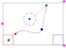
Fig. 7. Route re-planning after the opponent has been detected. The robot
travels from bottom left to top right position, its original route shown as
dotted line, new route as solid line
(screenshot)
8 Sensors and effectors
Our robot uses
several different types of sensors and effectors. For the Brain, all of them
are represented by objects which encapsulate their physical functionality and
provide communicational interface. The objects may even provide enhanced functionality
in addition to the straightforward feature passing.
The overall
software design is layered; currently it is composed of four layers. Fig. 8 gives an impression; the layers are in more detail
described in [2] and [8].
Currently used
effectors and sensors are:
- 2 Wheel power motors, 2 extractor
motors and 1 harvester motor (connected by one to 5 individual HBmotor boards);
- An encoders mounted on every motor
(connected to its respective HBmotor board);
- 2 bumpers located in front corners
of robot chassis (connected to both main wheel HBmotor boards);
- A bumper in the middle front area of
the robot for dispenser detection (can also provide the last detection of the
opponent);
- A compass; currently used only for
rough MCL samples weighting;
- A camera for detecting the colour of
a collected ball inside the robot;
- A camera for game elements lookup on
the playing field (it can look for the vertical dispensers as described earlier
or it can detect balls laying on the playfield);
Fig. 8. Control software design
- 3 active beacons located at fixed
positions around the playing field and 1 passive receiver mounted on the robot;
- We planned to use the exactly same
receiver to be placed on the opponent robot and transmit its data (i.e. the
opponent position) via Bluetooth to our robot, but we didn’t implement and tune
it early enough to use it during the contest. However, it could provide interesting
and important information
(It was also
possible to connect a regular keyboard or use network connection to the system
because the robot was run using standard Linux Operating system on a standard
miniITX board, but we do not consider these to be proper sensors for an autonomous
robot)
The robot main
hardware components are:
- Motherboard: VIA EPIA miniITX board with
512MB RAM and 2GB CompactFlash card.
- HBmotor board: Atmel ATmega8 microcontroller
+ standard MOSFET-type H-bridge.
- Power source: Sealed Pb
accumulators, 12V, 7.2Ah, 2.6kg.
- Motors: GHM-04 (7.2V, 0.7Nm at
0 rpm) with integrated gearbox 50:1 (giving output 175 rpm) + QME-01 encoders
(6000 steps per wheel revolution).
- Wheels: simple undamped wheels, 8.5 cm
diameter, max speed ~ 0.7 m/s.
- Ultrasonic sensors UST40T (transmitter)
and UST4R (receiver).
- CMPS03 compass.
10 Conclusion and Future Works
The current robot
design and implementation meet both the criteria determined by the Eurobot
contest rules and the expectations of the author team. Of course, as any other
project, it can be further enhanced and expanded, for example:
- The PID regulation could be
implemented in the HBmotor board. Its advantage is the speed of response it can
react to the changes. We expect faster reaching of the desired speed and
smoother motion of the robot.
- Currently the asynchronous state
switch is implemented so that when its handler finishes and the previous state
is to be restored, that state is restarted. For certain operations it might be
better to restore the previous state exactly from where it was paused. This
does not apply to all states (e.g. it makes sense when collecting the balls on
the playing field but it would not be useful for manoeuvring in front of the
dispenser) and it could be in fact used even now by splitting such states into
more smaller states. However, it would easily lead to very complicated state
machine.
- Many new sensors could be added
(more bumpers, GPS device for outdoor use, distance measuring sensors etc.).
- New actuators and manipulators can
be added to perform other tasks to those required for Eurobot contest.
Acknowledgements
The work was partly supported by the project
1ET100300419 of the Information Society Program of the National Research
Program of the
References
1. Eurobot Autonomous robot contest: http://www.eurobot.org
2. MART team internet homepage: http://mart.matfyz.cz
3.
Robotour
competition: http://robotika.cz/competitions/en
4. Intel OpenCV: http://www.intel.com/technology/computing/opencv/
5. F. Dellaert, D. Fox, W. Burgard, and
S. Thrun: Monte Carlo Localization for
6. CMPS03 Compass: http://www.robot-electronics.co.uk/acatalog/Compass.html